Test Functions
Table of contents
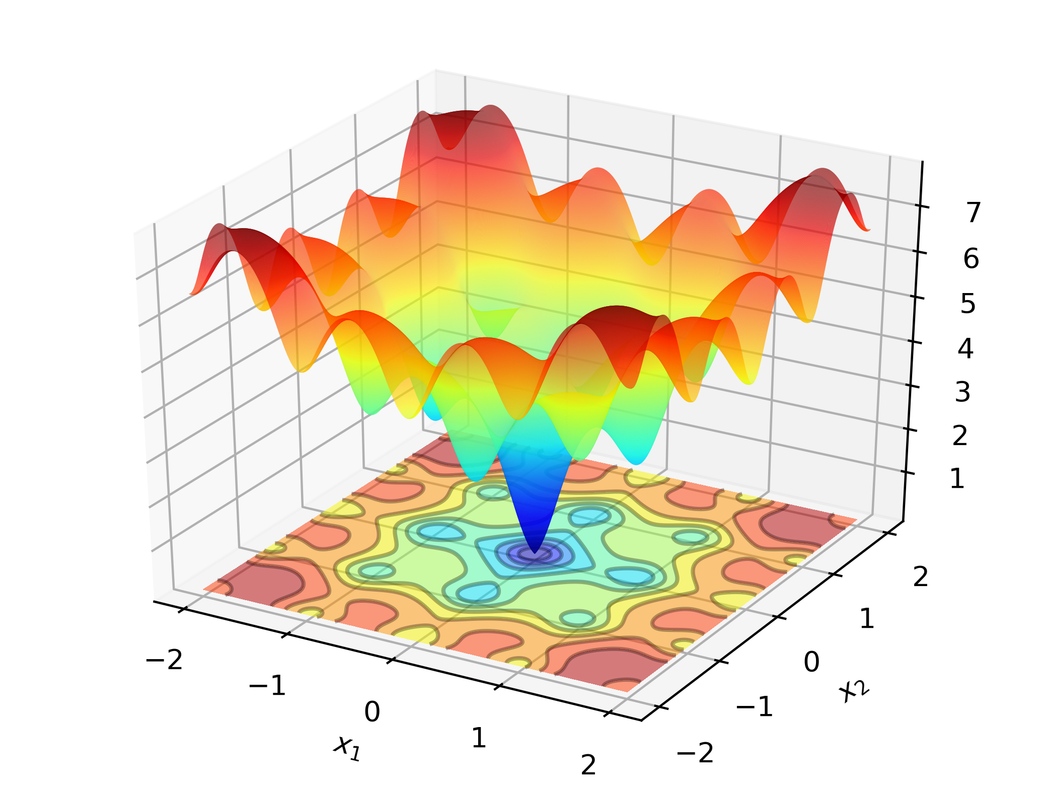
Ackley Function
The Ackley function is given by:
The minimum value is attained at \((0, 0)\).
A plot of the function is given below.
Code to run this example is given below.
Code (Click to show/hide)
#define OPTIM_PI 3.14159265358979

double
ackley_fn(const ColVec_t& vals_inp, ColVec_t* grad_out, void* opt_data)
{
    const double x = vals_inp(0);
    const double y = vals_inp(1);

    double obj_val = 20 + std::exp(1) - 20*std::exp( -0.2*std::sqrt(0.5*(x*x + y*y)) ) - std::exp( 0.5*(std::cos(2 * OPTIM_PI * x) + std::cos(2 * OPTIM_PI * y)) );

    return obj_val;
}
Beale Function
The Beale function is given by:
The minimum value is attained at \((3, 0.5)\). The function is non-convex.
The gradient is given by
The elements of the Hessian matrix are;
A plot of the function is given below.
Code to run this example is given below.
Code (Click to show/hide)
double
beale_fn(const ColVec_t& vals_inp, ColVec_t* grad_out, void* opt_data)
{
    const double x_1 = vals_inp(0);
    const double x_2 = vals_inp(1);

    // compute some terms only once

    const double x2sq = x_2 * x_2;
    const double x2cb = x2sq * x_2;
    const double x1x2 = x_1*x_2;

    //

    double obj_val = std::pow(1.5 - x_1 + x1x2, 2) + std::pow(2.25 - x_1 + x_1*x2sq, 2) + std::pow(2.625 - x_1 + x_1*x2cb, 2);

    if (grad_out) {
        (*grad_out)(0) = 2 * ( (1.5 - x_1 + x1x2)*(x_2 - 1) + (2.25 - x_1 + x_1*x2sq)*(x2sq - 1) + (2.625 - x_1 + x_1*x2cb)*(x2cb - 1)   );
        (*grad_out)(1) = 2 * ( (1.5 - x_1 + x1x2)*(x_1)     + (2.25 - x_1 + x_1*x2sq)*(2*x1x2)   + (2.625 - x_1 + x_1*x2cb)*(3*x_1*x2sq) );
    }

    return obj_val;
}
Booth Function
The Booth function is given by:
The minimum value is attained at \((1, 3)\).
The gradient (ignoring the box constraints) is given by
The hessian is given by
A plot of the function is given below.
Code to run this example is given below.
Code (Click to show/hide)
double
booth_fn(const ColVec_t& vals_inp, ColVec_t* grad_out, void* opt_data)
{
    double x_1 = vals_inp(0);
    double x_2 = vals_inp(1);

    double obj_val = std::pow(x_1 + 2*x_2 - 7.0, 2) + std::pow(2*x_1 + x_2 - 5.0, 2);

    if (grad_out) {
        (*grad_out)(0) = 10*x_1 + 8*x_2 - 34;
        (*grad_out)(1) = 8*x_1 + 10*x_2 - 38;
    }

    return obj_val;
}
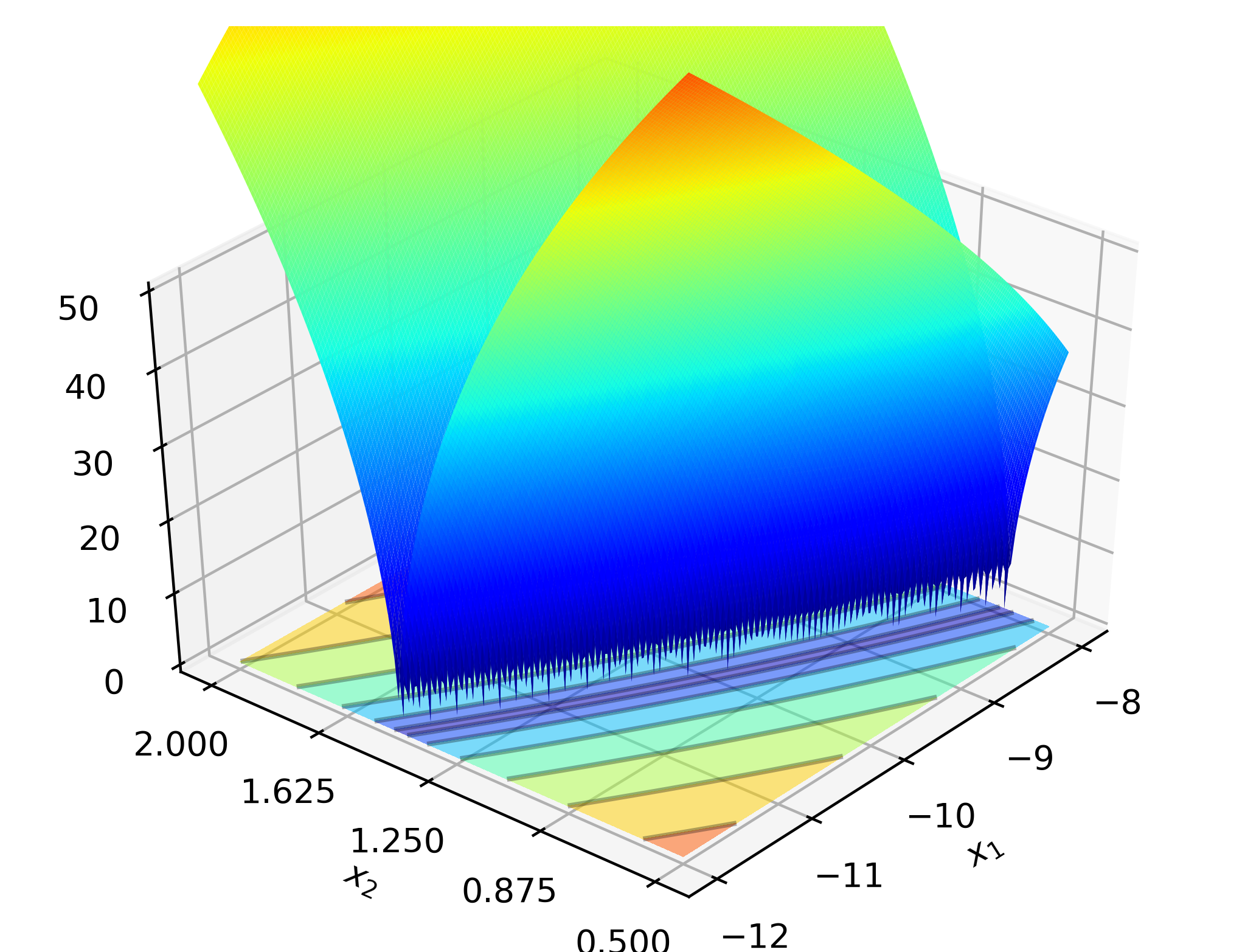
Bukin Function
The Bukin function (N. 6) is given by:
The minimum value is attained at \((-10, 1)\).
A plot of the function is given below.
Code to run this example is given below.
Code (Click to show/hide)
double
bukin_fn(const ColVec_t& vals_inp, ColVec_t* grad_out, void* opt_data)
{
    const double x = vals_inp(0);
    const double y = vals_inp(1);

    double obj_val = 100*std::sqrt(std::abs(y - 0.01*x*x)) + 0.01*std::abs(x + 10);

    return obj_val;
}
Levi Function
The Levi function (N. 13) is given by:
The minimum value is attained at \((1, 1)\).
A plot of the function is given below.
Code to run this example is given below.
Code (Click to show/hide)
#define OPTIM_PI 3.14159265358979

double
levi_fn(const ColVec_t& vals_inp, ColVec_t* grad_out, void* opt_data)
{
    const double x = vals_inp(0);
    const double y = vals_inp(1);
    const double pi = OPTIM_PI;

    double obj_val = std::pow( std::sin(3*pi*x), 2) + std::pow(x-1,2)*(1 + std::pow( std::sin(3 * OPTIM_PI * y), 2)) + std::pow(y-1,2)*(1 + std::pow( std::sin(2 * OPTIM_PI * x), 2));

    return obj_val;
}
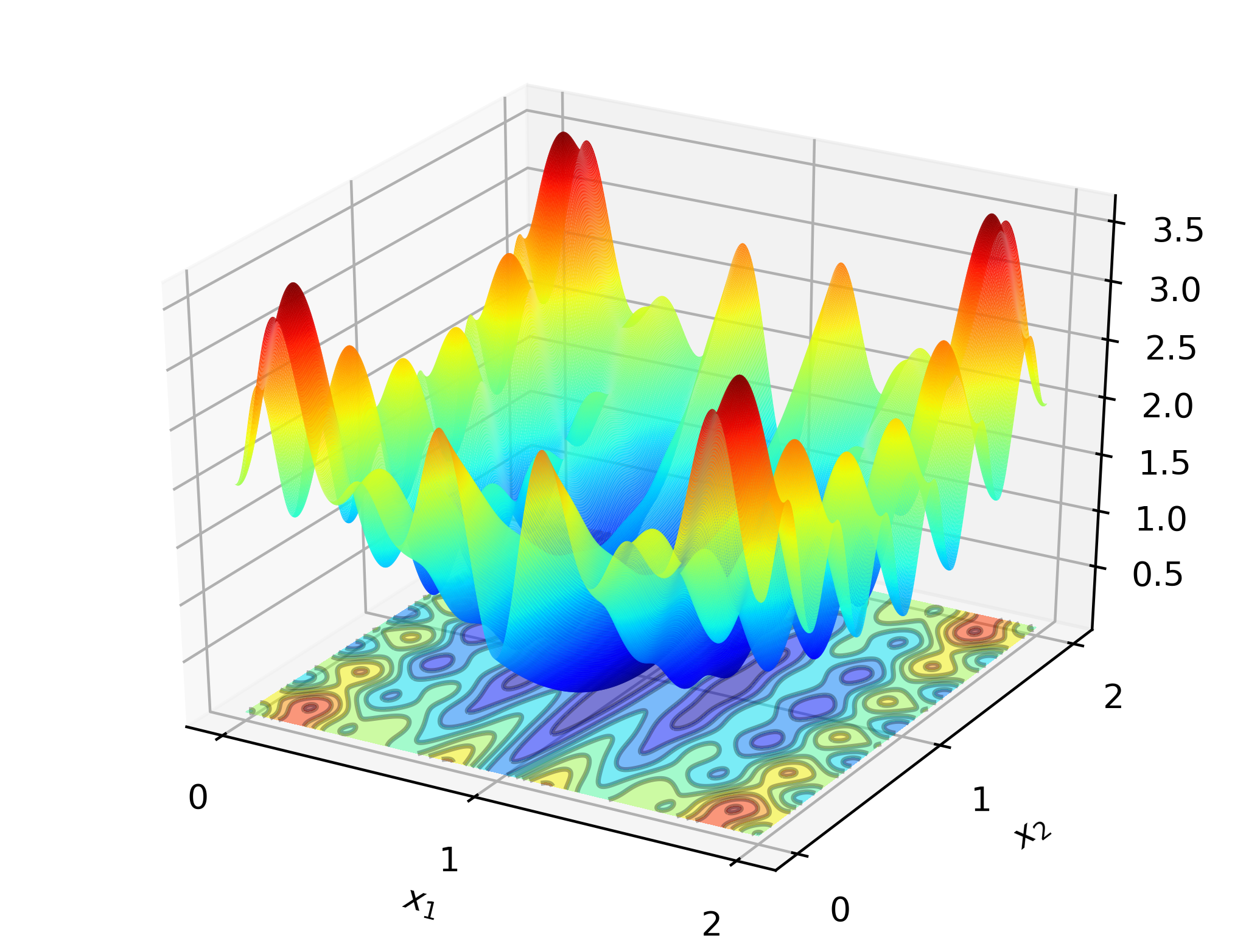
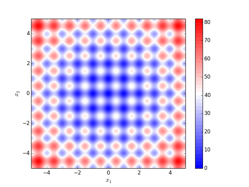
Rastrigin Function
The 2D Rastrigin function is given by:
The minimum value is attained at \((0, 0)\).
A plot of the function is given below.
Code to run this example is given below.
Code (Click to show/hide)
#define OPTIM_PI 3.14159265358979

double
rastrigin_fn(const ColVec_t& vals_inp, ColVec_t* grad_out, void* opt_data)
{
    const double x_1 = vals_inp(0);
    const double x_2 = vals_inp(1);

    double obj_val = 20 + x_1*x_1 + x_2*x_2 - 10 * (std::cos(2*OPTIM_PI*x_1) + std::cos(2*OPTIM_PI*x_2))

    return obj_val;
}
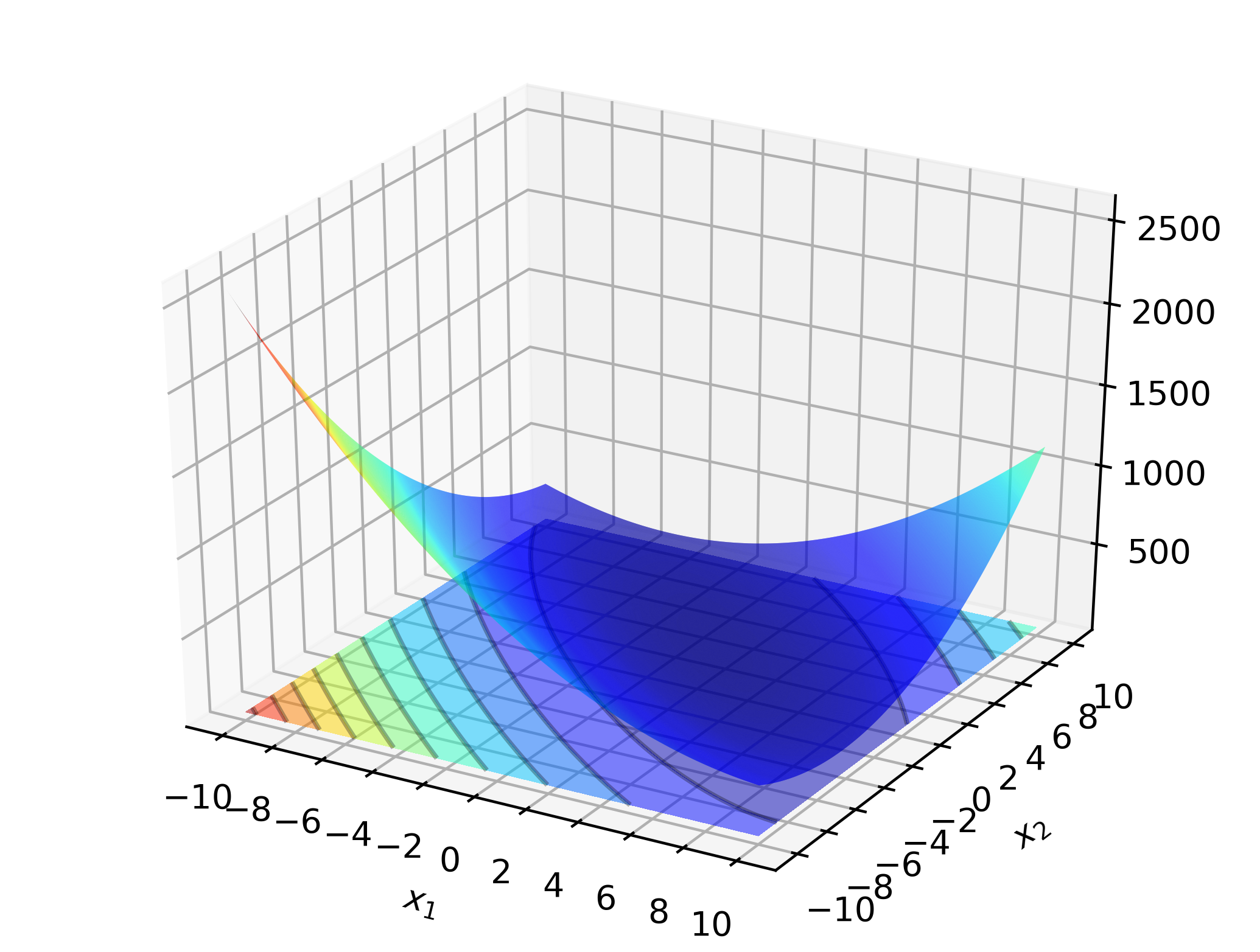
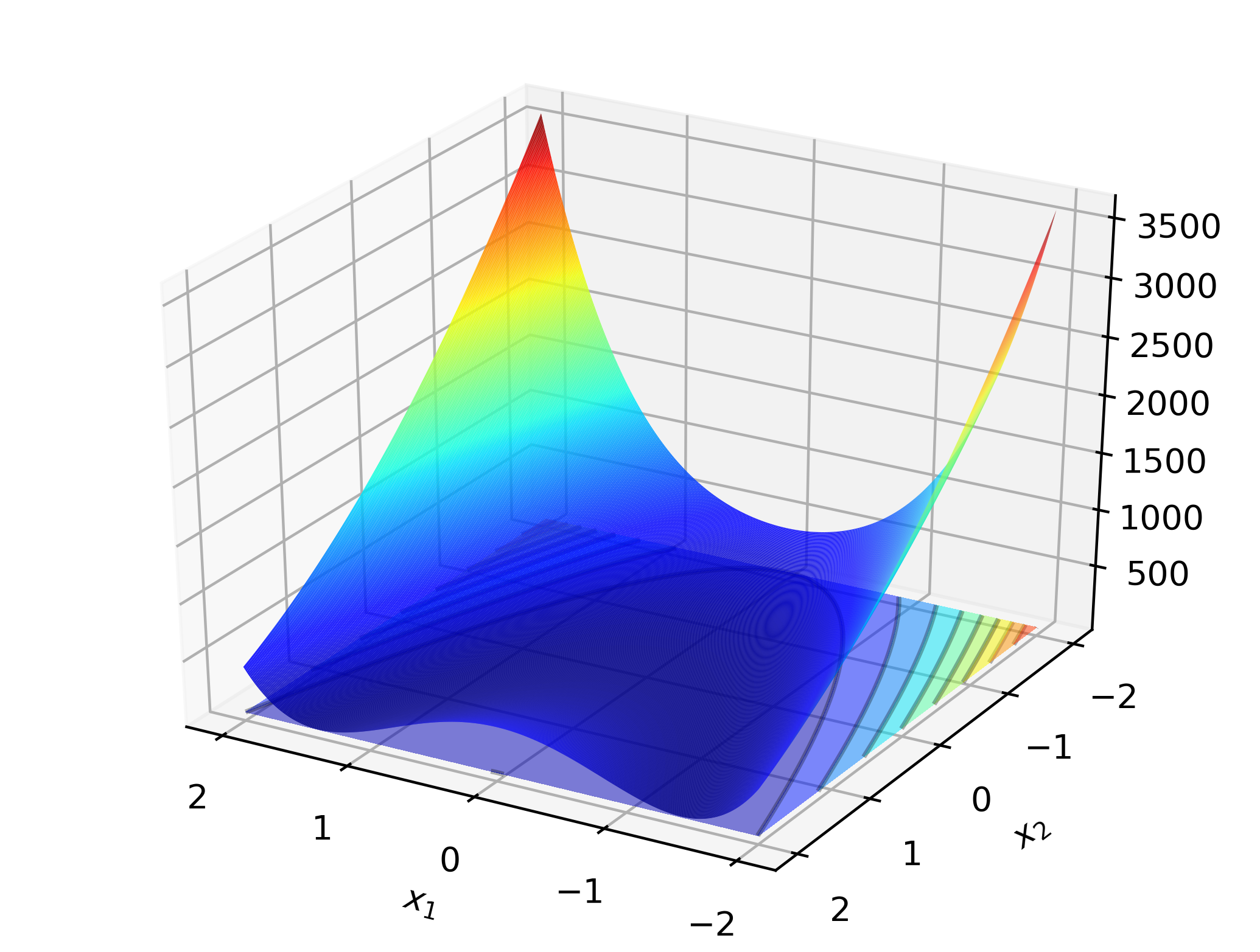
Rosenbrock Function
The 2D Rosenbrock function is given by:
The minimum value is attained at \((1, 1)\).
The gradient is given by
A plot of the function is given below.
Code to run this example is given below.
Code (Click to show/hide)
double
rosenbrock_fn(const ColVec_t& vals_inp, ColVec_t* grad_out, void* opt_data)
{
    const double x_1 = vals_inp(0);
    const double x_2 = vals_inp(1);

    const double x1sq = x_1 * x_1;

    double obj_val = 100*std::pow(x_2 - x1sq,2) + std::pow(1-x_1,2);

    if (grad_out) {
        (*grad_out)(0) = -400*(x_2 - x1sq)*x_1 - 2*(1-x_1);
        (*grad_out)(1) = 200*(x_2 - x1sq);
    }

    return obj_val;
}
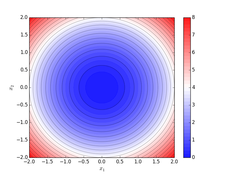
Sphere Function
The Sphere function is a very simple smooth test function, given by:
The minimum value is attained at the origin.
The gradient is given by
A contour plot of the Sphere function in two dimensions is given below.
Code to run this example is given below.
Armadillo (Click to show/hide)
#include "optim.hpp"

inline
double
sphere_fn(const arma::vec& vals_inp, arma::vec* grad_out, void* opt_data)
{
    double obj_val = arma::dot(vals_inp,vals_inp);

    if (grad_out) {
        *grad_out = 2.0*vals_inp;
    }

    return obj_val;
}

int main()
{
    const int test_dim = 5;

    arma::vec x = arma::ones(test_dim,1); // initial values (1,1,...,1)

    bool success = optim::bfgs(x, sphere_fn, nullptr);

    if (success) {
        std::cout << "bfgs: sphere test completed successfully." << "\n";
    } else {
        std::cout << "bfgs: sphere test completed unsuccessfully." << "\n";
    }

    arma::cout << "bfgs: solution to sphere test:\n" << x << arma::endl;

    return 0;
}
Eigen (Click to show/hide)
#include "optim.hpp"

inline
double
sphere_fn(const Eigen::VectorXd& vals_inp, Eigen::VectorXd* grad_out, void* opt_data)
{
    double obj_val = vals_inp.dot(vals_inp);

    if (grad_out) {
        *grad_out = 2.0*vals_inp;
    }

    return obj_val;
}

int main()
{
    const int test_dim = 5;

    Eigen::VectorXd x = Eigen::VectorXd::Ones(test_dim); // initial values (1,1,...,1)

    bool success = optim::bfgs(x, sphere_fn, nullptr);

    if (success) {
        std::cout << "bfgs: sphere test completed successfully." << "\n";
    } else {
        std::cout << "bfgs: sphere test completed unsuccessfully." << "\n";
    }

    std::cout << "bfgs: solution to sphere test:\n" << x << std::endl;

    return 0;
}
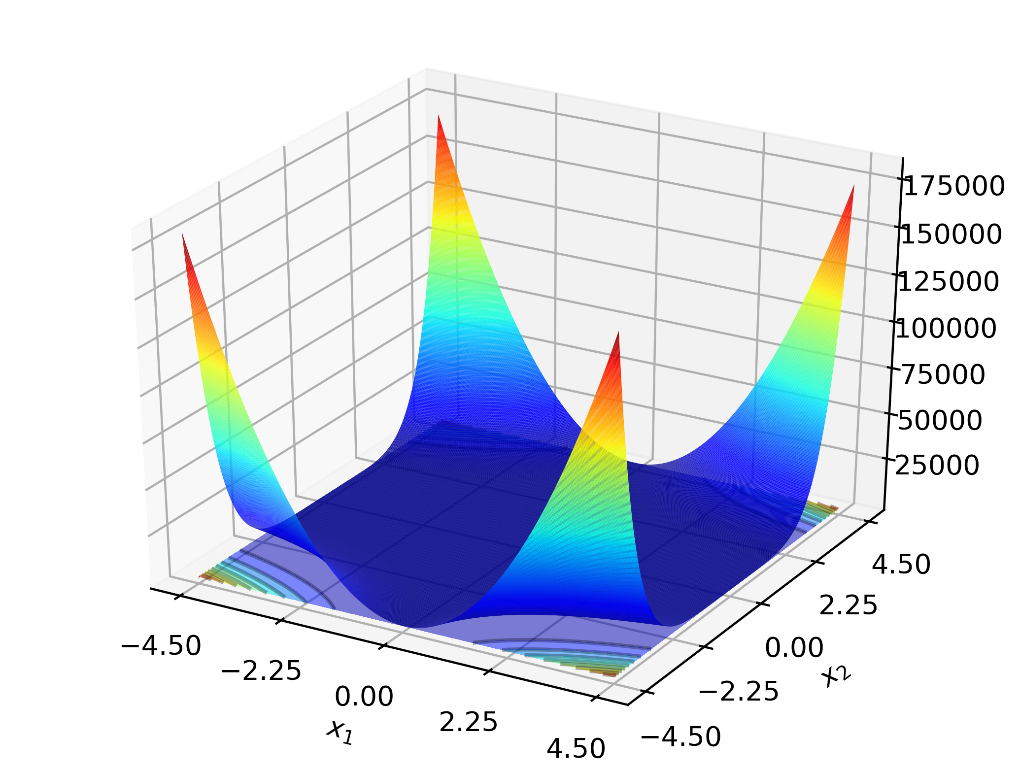
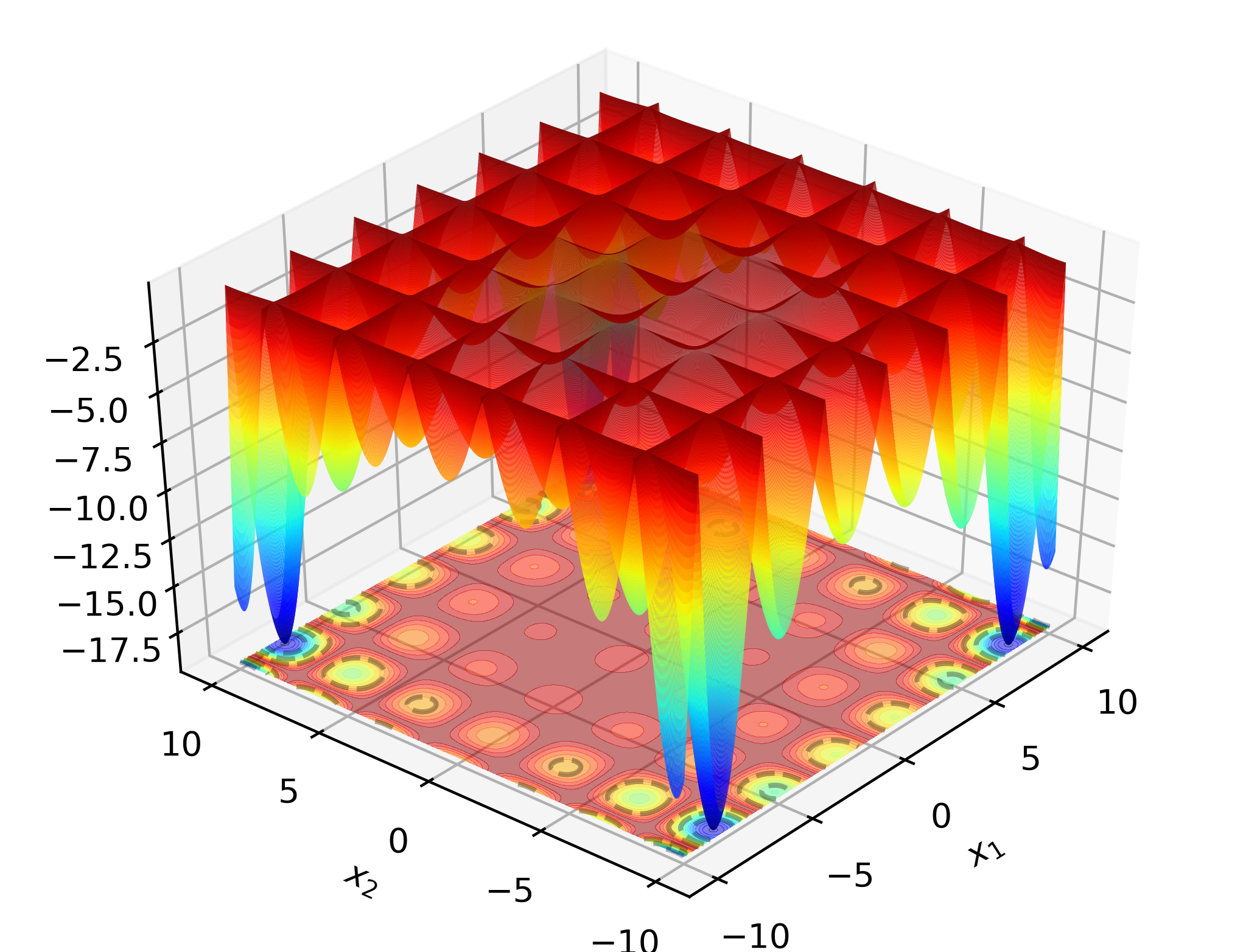
Table Function
The Hoelder Table function is given by:
The minimum value is attained at four locations: \((\pm 8.05502, \pm 9.66459)\).
A plot of the function is given below.
Code to run this example is given below.
Code (Click to show/hide)
#define OPTIM_PI 3.14159265358979

double
table_fn(const ColVec_t& vals_inp, ColVec_t* grad_out, void* opt_data)
{
    const double x = vals_inp(0);
    const double y = vals_inp(1);

    double obj_val = - std::abs( std::sin(x)*std::cos(y)*std::exp( std::abs( 1.0 - std::sqrt(x*x + y*y) / OPTIM_PI ) ) );

    return obj_val;
}